TensorFlow深度可分离卷积详解：tf.nn.depthwise_conv2d参数与实现

苏见山

发布时间：2026-10-13| 5人浏览过

原创

本文深入解析TensorFlow中tf.nn.depthwise_conv2d函数的实现原理。详细阐述其五个核心参数：input、filter、strides、padding和rate，并对比普通卷积与深度卷积在通道处理上的差异。通过构建自定义输入图像与卷积核的完整代码示例，直观展示深度卷积的计算过程与输出结果，帮助开发者理解并应用该技术在模型轻量化中的优势。

实验环境与功能概述

实验环境配置为TensorFlow 1.2.0版本，Python解释器版本为2.7。

功能概述

函数depthwise_conv2d源自深度可分离卷积（Depthwise Separable Convolutions）架构，该架构在提升模型效率方面表现显著。

相关研究参考Xception网络论文《Deep Learning with Depthwise Separable Convolutions》，该论文深入探讨了深度可分离卷积的应用。


tf.nn.depthwise_conv2d(input,filter,strides,padding,rate=None,name=None,data_format=None)

核心参数详解

除name参数用于指定操作名称外，data_format用于指定数据格式。与该方法直接相关的参数共有五个，具体如下。

input：表示需要进行卷积操作的输入图像，必须是一个4维Tensor，其形状符合[batch, height, width, in_channels]的定义。具体含义为[训练时一个batch的图片数量, 图片高度, 图片宽度, 图像通道数]。

filter：相当于CNN中的卷积核，同样要求是一个4维Tensor，形状符合[filter_height, filter_width, in_channels, channel_multiplier]的定义。具体含义为[卷积核的高度，卷积核的宽度，输入通道数，输出卷积乘子]。需要注意的是，这里的第三维in_channels与参数value的第四维相对应。

strides：定义卷积操作在图像上滑动的步长。

padding：字符串类型的参数，取值只能是”SAME”或”VALID”之一，该值决定了边缘填充的具体方式。

rate：关于该参数的详细解释，可参考【Tensorflow】tf.nn.atrous_conv2d如何实现空洞卷积？一文。

函数返回一个Tensor，其形状为[batch, out_height, out_width, in_channels * channel_multiplier]。需注意，输出通道数变为in_channels * channel_multiplier，即输入通道数与通道乘子的乘积。

深度卷积实验与原理分析

实验验证

为了直观展示depthwise_conv2d的工作机制，我们需要构建自定义的输入图像和卷积核数据。


img1 = tf.constant(value=[[[[1],[2],[3],[4]],[[1],[2],[3],[4]],[[1],[2],[3],[4]],[[1],[2],[3],[4]]]],dtype=tf.float32)
img2 = tf.constant(value=[[[[1],[1],[1],[1]],[[1],[1],[1],[1]],[[1],[1],[1],[1]],[[1],[1],[1],[1]]]],dtype=tf.float32)
img = tf.concat(values=[img1,img2],axis=3)


filter1 = tf.constant(value=0, shape=[3,3,1,1],dtype=tf.float32)
filter2 = tf.constant(value=1, shape=[3,3,1,1],dtype=tf.float32)
filter3 = tf.constant(value=2, shape=[3,3,1,1],dtype=tf.float32)
filter4 = tf.constant(value=3, shape=[3,3,1,1],dtype=tf.float32)
filter_out1 = tf.concat(values=[filter1,filter2],axis=2)
filter_out2 = tf.concat(values=[filter3,filter4],axis=2)
filter = tf.concat(values=[filter_out1,filter_out2],axis=3)

完成img和filter的构建后，即可执行卷积操作。


out_img = tf.nn.conv2d(input=img, filter=filter, strides=[1,1,1,1], padding='VALID')

下面通过一张图示详细展示这一计算过程。

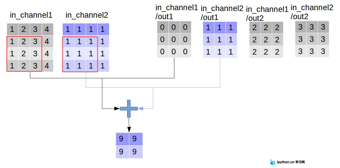
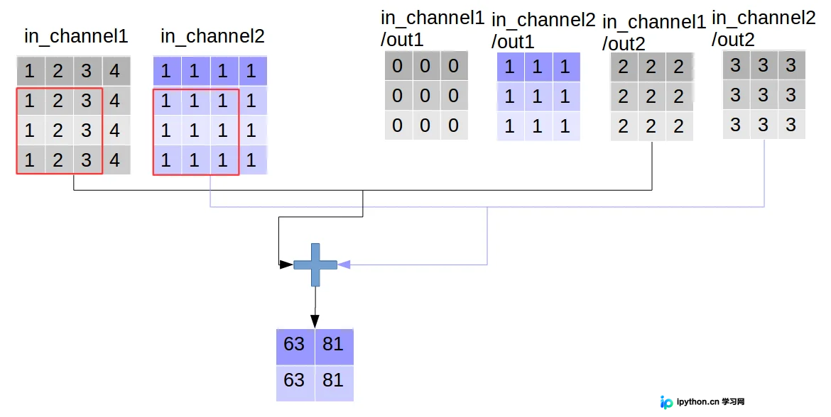
这是普通卷积的处理流程，接下来我们对比查看深度卷积的效果。


out_img = tf.nn.depthwise_conv2d(input=img, filter=filter, strides=[1,1,1,1], rate=[1,1], padding='VALID')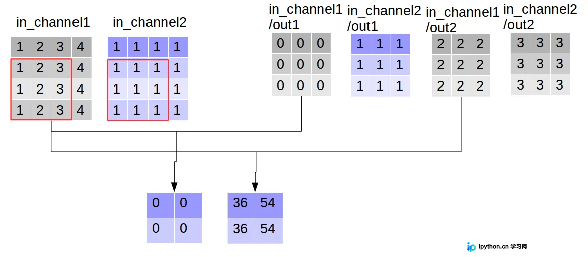

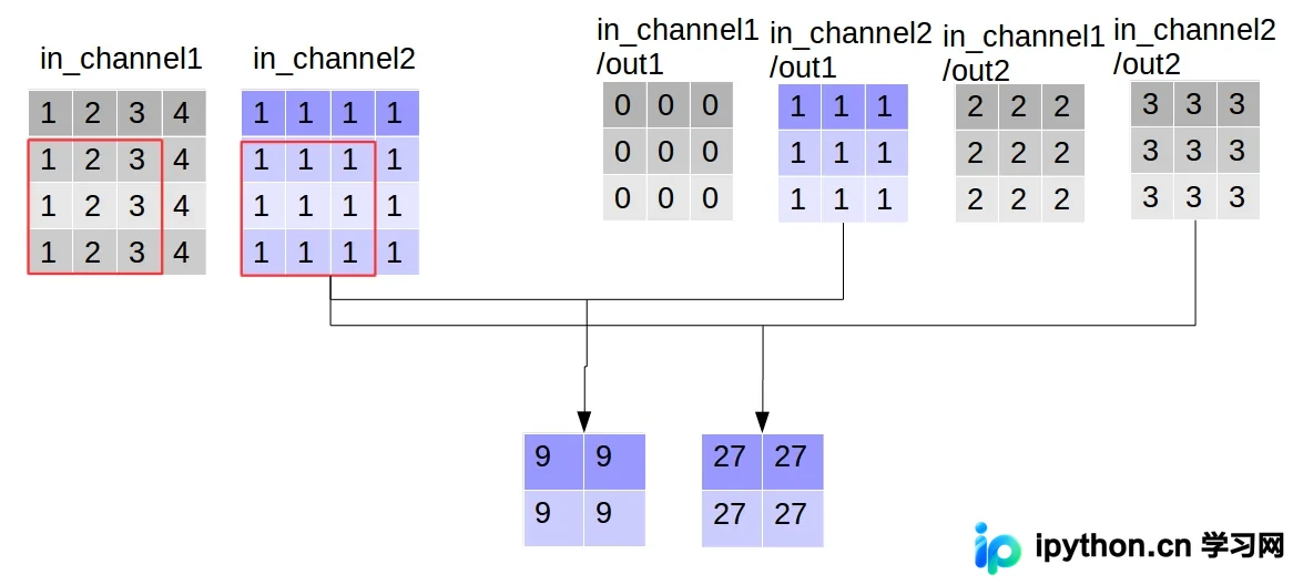
现在可以形象地解释depthwise_conv2d卷积的原理。在普通卷积中，我们对卷积核每一个out_channel的两个通道分别与输入的两个通道做卷积并相加，从而得到feature map的一个channel。而在depthwise_conv2d卷积中，我们对每一个对应的in_channel分别进行卷积，生成两个out_channel。因此，获得的feature map的通道数量可以用in_channel* channel_multiplier来表达，这里的channel_multiplier即为卷积核的第四维（channel_multiplier）。

代码实现与结果展示

代码清单


import tensorflow as tf


img1 = tf.constant(value=[[[[1],[2],[3],[4]],[[1],[2],[3],[4]],[[1],[2],[3],[4]],[[1],[2],[3],[4]]]],dtype=tf.float32)
img2 = tf.constant(value=[[[[1],[1],[1],[1]],[[1],[1],[1],[1]],[[1],[1],[1],[1]],[[1],[1],[1],[1]]]],dtype=tf.float32)
img = tf.concat(values=[img1,img2],axis=3)
filter1 = tf.constant(value=0, shape=[3,3,1,1],dtype=tf.float32)
filter2 = tf.constant(value=1, shape=[3,3,1,1],dtype=tf.float32)
filter3 = tf.constant(value=2, shape=[3,3,1,1],dtype=tf.float32)
filter4 = tf.constant(value=3, shape=[3,3,1,1],dtype=tf.float32)
filter_out1 = tf.concat(values=[filter1,filter2],axis=2)
filter_out2 = tf.concat(values=[filter3,filter4],axis=2)
filter = tf.concat(values=[filter_out1,filter_out2],axis=3)

out_img = tf.nn.depthwise_conv2d(input=img, filter=filter, strides=[1,1,1,1], rate=[1,1], padding='VALID')

输出结果：