Python生成非均匀随机数的三种算法:反变换法与舍选抽样详解

本文介绍Python中生成非均匀随机数的三种方法:反变换法、基本舍选抽样法及推广舍选抽样法。通过具体代码示例,演示如何利用numpy和matplotlib实现从[0,6]和[0,10]区间的指数分布采样,并对比各方法的运算步数与效率,帮助开发者选择最优算法。
1.反变换法
假设需要生成服从分布函数F(x)的连续随机变量X。若已拥有[0,1]区间上的均匀分布随机数R,则可通过反变换公式生成X:
即F(x)=r,解得x=F-1(r)
反函数存在的条件是:若函数y=f(x)在定义域D上单调,则其反函数必然存在且同样单调。由于分布函数F(x)是单调递增的,因此其反函数存在。从直观角度理解,因为r与x一一对应,且对于[0,1]均匀分布随机数R,P(R≤r)=r。因此,连续随机数X≤x的概率P(X≤x)等于P(R≤r),即等于r=F(x)。
这表明X的分布函数确为F(x)。
示例:以下代码利用反变换法在区间[0, 6]上生成随机数,其概率密度近似为P(x)=e^-x
import numpy as np
import matplotlib.pyplot as plt
# probability distribution we're trying to calculate
p = lambda x: np.exp(-x)
# CDF of p
CDF = lambda x: 1-np.exp(-x)
# invert the CDF
invCDF = lambda x: -np.log(1-x)
# domain limits
xmin = 0 # the lower limit of our domain
xmax = 6 # the upper limit of our domain
# range limits
rmin = CDF(xmin)
rmax = CDF(xmax)
N = 10000 # the total of samples we wish to generate
# generate uniform samples in our range then invert the CDF
# to get samples of our target distribution
R = np.random.uniform(rmin, rmax, N)
X = invCDF(R)
# get the histogram info
hinfo = np.histogram(X,100)
# plot the histogram
plt.hist(X,bins=100, label=u'Samples');
# plot our (normalized) function
xvals=np.linspace(xmin, xmax, 1000)
plt.plot(xvals, hinfo[0][0]*p(xvals), 'r', label=u'p(x)')
# turn on the legend
plt.legend()
plt.show()
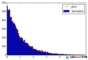
通常情况下,直方图的外轮廓曲线会逼近总体X的概率密度曲线。
2.舍选抽样法(Rejection Method)
在使用反变换法时,若无法求出F-1(x)的解析形式或F(x)本身无解析形式,可尝试使用F-1(x)的近似公式。然而,由于反函数计算量较大,这种方法有时并不适用。另一种由Von Neumann提出的方法是舍选抽样法。下图中曲线w(x)表示概率密度函数,按该密度函数生成随机数的步骤如下:
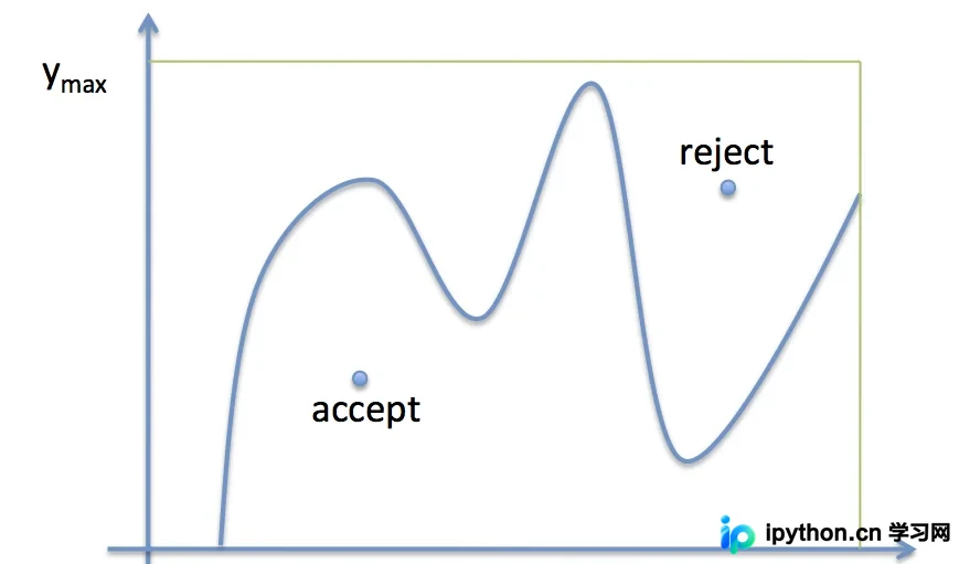
基本舍选抽样法的步骤如下:
1. 在[xmin, xmax]区间内均匀抽取x
2. 在[0, ymax]区间内均匀抽取y
3. 若y < w(x),则接受该样本;否则拒绝
4. 重复上述过程
即落在曲线w(x)与X轴围成区域内的点被接受,区域外的点被舍弃。
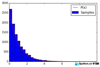
示例:以下代码使用基本舍选抽样法在区间[0, 10]上生成随机数,其概率密度近似为P(x)=e^-x
# -*- coding: utf-8 -*-
'''
The following code produces samples that follow the distribution P(x)=e^−x
for x=[0, 10] and generates a histogram of the sampled distribution.
'''
import numpy as np
import matplotlib.pyplot as plt
P = lambda x: np.exp(-x)
# domain limits
xmin = 0 # the lower limit of our domain
xmax = 10 # the upper limit of our domain
# range limit (supremum) for y
ymax = 1
N = 10000  # the total of samples we wish to generate
accepted = 0 # the number of accepted samples
samples = np.zeros(N)
count = 0  # the total count of proposals
# generation loop
while (accepted < N):
    # pick a uniform number on [xmin, xmax) (e.g. 0...10)
  x = np.random.uniform(xmin, xmax)
    # pick a uniform number on [0, ymax)
  y = np.random.uniform(0,ymax)
    # Do the accept/reject comparison
  if y < P(x):
    samples[accepted] = x
    accepted += 1
    count +=1
  print count, accepted
# get the histogram info
# If bins is an int, it defines the number of equal-width bins in the given range
(n, bins)= np.histogram(samples, bins=30) # Returns: n-The values of the histogram,n是直方图中柱子的高度
# plot the histogram
plt.hist(samples,bins=30,label=u'Samples')  # bins=30即直方图中有30根柱子
# plot our (normalized) function
xvals=np.linspace(xmin, xmax, 1000)
plt.plot(xvals, n[0]*P(xvals), 'r', label=u'P(x)')
# turn on the legend
plt.legend()
plt.show()
>>>
99552 10000
3.推广的舍选抽样法
从上图可以看出,基本舍选抽样法的效率较低,因为随机数x和y分别在区间[xmin, xmax]和[0, ymax]上均匀分布,大部分点不会落在w(x)曲线之下(由于e^-x曲线形状一边高一边低,其曲线下面积占矩形面积的比例很小,导致舍选效率低下)。为了提高简单舍选抽样法的效率,可以构造一个新的密度函数q(x)(称为建议分布,从中可以方便地抽取样本),使其形状接近p(x),并选择一个常数k使得kq(x)≥w(x)对定义域内的所有x成立。对应下图,首先从分布q(z)中生成随机数z0,然后按均匀分布从区间[0, kq(z0)]生成一个随机数u0。若u0 > p(z0),则拒绝该样本;否则保留u0。即下图中灰色区域内的点都要舍弃。可见,由于随机点u0仅出现在曲线kq(x)之下,且在q(x)较大处出现频率较高,从而显著提高了采样效率。显然,q(x)的形状越接近p(x),采样效率越高。
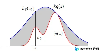
根据上述思想,采样规则也可表述如下:
1. 从建议分布q(x)中抽取x
2. 在[0, 1]区间内均匀抽取y
3. 若y < p(x)/kq(x),则接受样本;否则拒绝
4. 重复上述过程
以下示例中选择函数p(x)=1/(x+1)作为建议分布,k=1。曲线1/(x+1)的形状与e^-x相近。
import numpy as np
import matplotlib.pyplot as plt
p = lambda x: np.exp(-x)     # our distribution
g = lambda x: 1/(x+1)      # our proposal pdf (we're choosing k to be 1)
CDFg = lambda x: np.log(x +1)  # generates our proposal using inverse sampling
# domain limits
xmin = 0 # the lower limit of our domain
xmax = 10 # the upper limit of our domain
# range limits for inverse sampling
umin = CDFg(xmin)
umax = CDFg(xmax)
N = 10000 # the total of samples we wish to generate
accepted = 0 # the number of accepted samples
samples = np.zeros(N)
count = 0 # the total count of proposals
# generation loop
while (accepted < N):
    # Sample from g using inverse sampling
  u = np.random.uniform(umin, umax)
  xproposal = np.exp(u) - 1
  # pick a uniform number on [0, 1)
  y = np.random.uniform(0, 1)
  # Do the accept/reject comparison
  if y < p(xproposal)/g(xproposal):
    samples[accepted] = xproposal
    accepted += 1
    count +=1
  print count, accepted
# get the histogram info
hinfo = np.histogram(samples,50)
# plot the histogram
plt.hist(samples,bins=50, label=u'Samples');
# plot our (normalized) function
xvals=np.linspace(xmin, xmax, 1000)
plt.plot(xvals, hinfo[0][0]*p(xvals), 'r', label=u'p(x)')
# turn on the legend
plt.legend()
plt.show()
>>>
24051 10000
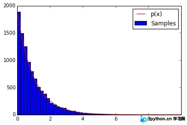
对比基本舍选法和改进舍选法的结果,前者生成符合分布要求的10000个随机数需运算99552步,后者仅需24051步,可见效率得到显著提升。
总结
以上即为本文关于Python生成非均匀随机数的几种方法及代码分享的全部内容,希望对大家有所帮助。感兴趣的朋友可以继续参阅本站:
Python数据可视化编程通过Matplotlib创建散点图代码示例
Python编程实现使用线性回归预测数据
Python数据可视化正态分布简单分析及实现代码
如有不足之处,欢迎留言指出。感谢朋友们对本站的支持!
免责声明:本文内容仅供参考,不代表本站观点。转载或引用请注明出处。