Python实现随机梯度下降法:原理与代码详解

本文深入解析随机梯度下降法(SGD)的核心思想,对比传统梯度下降法在大数据集下的性能瓶颈。通过推导权值更新公式,阐述SGD如何利用单样本近似梯度以加速收敛并跳出局部最优。附带Python完整实现代码,展示从数据构造到模型训练的全过程,帮助开发者掌握这一关键优化算法。
在深入阅读本文之前,建议先回顾上一篇关于Python实现梯度下降法的文章,以便更好地理解两者的联系与区别。
一、为什么需要随机梯度下降算法
请注意梯度下降法中权值的更新机制(具体推导过程已在上一篇文章中详述)。
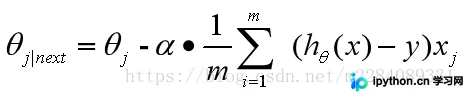
这意味着每次更新权值 时,都需要遍历整个数据集(注意公式中的求和符号)。当数据量较小时,这种算法尚可接受;然而,一旦数据规模庞大,该方法会导致收敛过程极其缓慢。此外,当损失函数存在多个局部极小值时,传统梯度下降法无法保证搜索到全局最优解。为解决上述问题,引入了梯度下降法的改进版本:随机梯度下降法。
二、核心思想
在权值更新策略上,随机梯度下降法不再遍历全部数据集,而是每次仅选取一个样本进行计算(对于程序员而言,这通常意味着需要一个随机函数来随机选择一个样本)。一般而言,其步长选择比传统梯度下降法更小。这是因为传统梯度下降法使用的是精确梯度,因此在凸问题中可以朝着全局最优解进行较大步长的迭代;而随机梯度下降法使用的是近似梯度,有时甚至可能偏离真正的梯度下降方向,因此其迭代过程较为缓慢。然而,这种特性带来的好处是:相比传统梯度下降法,随机梯度下降法更不容易陷入局部最优解。
三、权值更新方式
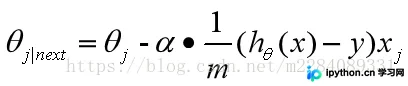
(其中i表示样本标号下标,j表示样本维数下标)
四、代码实现(整体逻辑与梯度下降法相似,主要区别在于while循环内部的处理逻辑)。
import numpy as np
import matplotlib.pyplot as plt
from mpl_toolkits.mplot3d import axes3d
from matplotlib import style


#构造数据
def get_data(sample_num=1000):
 """
 拟合函数为
 y = 5*x1 + 7*x2
 :return:
 """
 x1 = np.linspace(0, 9, sample_num)
 x2 = np.linspace(4, 13, sample_num)
 x = np.concatenate(([x1], [x2]), axis=0).T
 y = np.dot(x, np.array([5, 7]).T)
 return x, y
#梯度下降法
def SGD(samples, y, step_size=2, max_iter_count=1000):
 """
 :param samples: 样本
 :param y: 结果value
 :param step_size: 每一接迭代的步长
 :param max_iter_count: 最大的迭代次数
 :param batch_size: 随机选取的相对于总样本的大小
 :return:
 """
 #确定样本数量以及变量的个数初始化theta值

 m, var = samples.shape
 theta = np.zeros(2)
 y = y.flatten()
 #进入循环内
 loss = 1
 iter_count = 0
 iter_list=[]
 loss_list=[]
 theta1=[]
 theta2=[]
 #当损失精度大于0.01且迭代此时小于最大迭代次数时,进行
 while loss > 0.01 and iter_count < max_iter_count:
 loss = 0
 #梯度计算
 theta1.append(theta[0])
 theta2.append(theta[1])
 #样本维数下标
 rand1 = np.random.randint(0,m,1)
 h = np.dot(theta,samples[rand1].T)
 #关键点,只需要一个样本点来更新权值
 for i in range(len(theta)):
 theta[i] =theta[i] - step_size*(1/m)*(h - y[rand1])*samples[rand1,i]
 #计算总体的损失精度,等于各个样本损失精度之和
 for i in range(m):
 h = np.dot(theta.T, samples[i])
 #每组样本点损失的精度
 every_loss = (1/(var*m))*np.power((h - y[i]), 2)
 loss = loss + every_loss

 print("iter_count: ", iter_count, "the loss:", loss)

 iter_list.append(iter_count)
 loss_list.append(loss)

 iter_count += 1
 plt.plot(iter_list,loss_list)
 plt.xlabel("iter")
 plt.ylabel("loss")
 plt.show()
 return theta1,theta2,theta,loss_list

def painter3D(theta1,theta2,loss):
 style.use('ggplot')
 fig = plt.figure()
 ax1 = fig.add_subplot(111, projection='3d')
 x,y,z = theta1,theta2,loss
 ax1.plot_wireframe(x,y,z, rstride=5, cstride=5)
 ax1.set_xlabel("theta1")
 ax1.set_ylabel("theta2")
 ax1.set_zlabel("loss")
 plt.show()

if __name__ == '__main__':
 samples, y = get_data()
 theta1,theta2,theta,loss_list = SGD(samples, y)
 print(theta) # 会很接近[5, 7]

 painter3D(theta1,theta2,loss_list)
以上就是本文的全部内容,希望能为您的学习提供有益的帮助,也欢迎大家继续支持本站。
免责声明:本文内容仅供参考,不代表本站观点。转载或引用请注明出处。