Python实现梯度下降算法详解：从SymPy符号计算到3D可视化

周末不加班

发布时间：2026-10-14| 5人浏览过

原创

本文详细介绍如何使用Python实现梯度下降算法。通过SymPy库进行符号变量定义与偏导数自动求解，结合Matplotlib绘制3D散点图与拟合平面，直观验证算法结果。文章涵盖Python版本选择、数据集构建及核心代码实现，适合机器学习初学者参考。

环境配置与数据集准备

Python版本选择

本例选用Python 2.7版本。此前尝试Python 3时，在绘制3D图形环节出现报错，为确保可视化功能正常运行，故回退至Python 2.7环境。

数据集选择

选取包含两个自变量及三个待估参数的数据集，旨在通过构建3D图形对算法输出结果进行直观验证。

SymPy符号计算核心函数解析

部分函数总结

symbols()函数：使用前需确保已安装sympy库。具体用法如下：


>>> x1 = symbols('x2')
>>> x1 + 1
x2 + 1

在此示例中，x1与x2存在本质区别：x2专指代函数中的变量，而x1作为Python普通变量，既可用于表示函数变量，也可代表其他任意量，并在计算中替代x2。实际编程时，虽可将x1和x2均命名为x，但需明确二者在语义上的差异。参考以下示例：


>>> x = symbols('x')
>>> expr = x + 1
>>> x = 2
>>> print(expr)
x + 1

当Python变量x被数值2覆盖后，它不再表示函数变量x，但表达式expr仍保持为函数变量x+1的别名，因此打印结果仍为x+1。 subs()函数：鉴于常规赋值方式无法直接为函数变量赋值，SymPy提供了专门函数实现此功能，用法如下：


>>> (1 + x*y).subs(x, pi)#一个参数时的用法
pi*y + 1
>>> (1 + x*y).subs({x:pi, y:2})#多个参数时的用法
1 + 2*pi

diff()函数：用于计算偏导数。调用格式为result=diff(fun,x)，即求fun函数对变量x的偏导数。注意，返回的result仍为变量对象，需通过赋值或代入具体数值才能获得精确结果。

梯度下降算法完整代码实现

代码实现：


from __future__ import division
from sympy import symbols, diff, expand
import numpy as np
import matplotlib.pyplot as plt
from mpl_toolkits.mplot3d import Axes3D

data = {'x1': [100, 50, 100, 100, 50, 80, 75, 65, 90, 90],
        'x2': [4, 3, 4, 2, 2, 2, 3, 4, 3, 2],
        'y': [9.3, 4.8, 8.9, 6.5, 4.2, 6.2, 7.4, 6.0, 7.6, 6.1]}#初始化数据集
theta0, theta1, theta2 = symbols('theta0 theta1 theta2', real=True)  # y=theta0+theta1*x1+theta2*x2,定义参数
costfuc = 0 * theta0
for i in range(10):
    costfuc += (theta0 + theta1 * data['x1'][i] + theta2 * data['x2'][i] - data['y'][i]) ** 2
costfuc /= 20#初始化代价函数
dtheta0 = diff(costfuc, theta0)
dtheta1 = diff(costfuc, theta1)
dtheta2 = diff(costfuc, theta2)

rtheta0 = 1
rtheta1 = 1
rtheta2 = 1#为参数赋初始值

costvalue = costfuc.subs({theta0: rtheta0, theta1: rtheta1, theta2: rtheta2})
newcostvalue = 0#用cost的值的变化程度来判断是否已经到最小值了
count = 0
alpha = 0.0001#设置学习率，一定要设置的比较小，否则无法到达最小值
while (costvalue - newcostvalue > 0.00001 or newcostvalue - costvalue > 0.00001) and count < 1000:
    count += 1
    costvalue = newcostvalue
    rtheta0 = rtheta0 - alpha * dtheta0.subs({theta0: rtheta0, theta1: rtheta1, theta2: rtheta2})
    rtheta1 = rtheta1 - alpha * dtheta1.subs({theta0: rtheta0, theta1: rtheta1, theta2: rtheta2})
    rtheta2 = rtheta2 - alpha * dtheta2.subs({theta0: rtheta0, theta1: rtheta1, theta2: rtheta2})
    newcostvalue = costfuc.subs({theta0: rtheta0, theta1: rtheta1, theta2: rtheta2})
rtheta0 = round(rtheta0, 4)
rtheta1 = round(rtheta1, 4)
rtheta2 = round(rtheta2, 4)#给结果保留4位小数，防止数值溢出
print(rtheta0, rtheta1, rtheta2)

fig = plt.figure()
ax = Axes3D(fig)
ax.scatter(data['x1'], data['x2'], data['y'])  # 绘制散点图
xx = np.arange(20, 100, 1)
yy = np.arange(1, 5, 0.05)
X, Y = np.meshgrid(xx, yy)
Z = X * rtheta1 + Y * rtheta2 + rtheta0
ax.plot_surface(X, Y, Z, rstride=1, cstride=1, cmap=plt.get_cmap('rainbow'))

plt.show()#绘制3d图进行验证

运行结果：

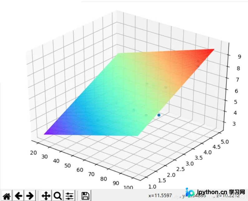
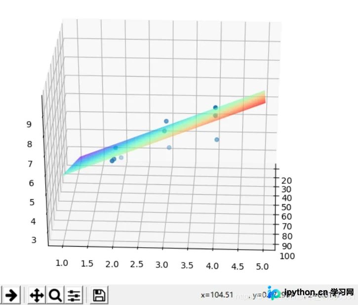
实例扩展：


'''
梯度下降算法
Batch Gradient Descent
Stochastic Gradient Descent SGD
'''
__author__ = 'epleone'
import numpy as np
import matplotlib.pyplot as plt
from mpl_toolkits.mplot3d import Axes3D
import sys

# 使用随机数种子， 让每次的随机数生成相同，方便调试
# np.random.seed(111111111)


class GradientDescent(object):
 eps = 1.0e-8
 max_iter = 1000000 # 暂时不需要
 dim = 1
 func_args = [2.1, 2.7] # [w_0, .., w_dim, b]

 def __init__(self, func_arg=None, N=1000):
 self.data_num = N
 if func_arg is not None:
 self.FuncArgs = func_arg
 self._getData()

 def _getData(self):
 x = 20 * (np.random.rand(self.data_num, self.dim) - 0.5)
 b_1 = np.ones((self.data_num, 1), dtype=np.float)
 # x = np.concatenate((x, b_1), axis=1)
 self.x = np.concatenate((x, b_1), axis=1)

 def func(self, x):
 # noise太大的话， 梯度下降法失去作用
 noise = 0.01 * np.random.randn(self.data_num) + 0
 w = np.array(self.func_args)
 # y1 = w * self.x[0, ] # 直接相乘
 y = np.dot(self.x, w) # 矩阵乘法
 y += noise
 return y

 @property
 def FuncArgs(self):
 return self.func_args

 @FuncArgs.setter
 def FuncArgs(self, args):
 if not isinstance(args, list):
 raise Exception(
 'args is not list, it should be like [w_0, ..., w_dim, b]')
 if len(args) == 0:
 raise Exception('args is empty list!!')
 if len(args) == 1:
 args.append(0.0)
 self.func_args = args
 self.dim = len(args) - 1
 self._getData()

 @property
 def EPS(self):
 return self.eps

 @EPS.setter
 def EPS(self, value):
 if not isinstance(value, float) and not isinstance(value, int):
 raise Exception("The type of eps should be an float number")
 self.eps = value

 def plotFunc(self):
 # 一维画图
 if self.dim == 1:
 # x = np.sort(self.x, axis=0)
 x = self.x
 y = self.func(x)
 fig, ax = plt.subplots()
 ax.plot(x, y, 'o')
 ax.set(xlabel='x ', ylabel='y', title='Loss Curve')
 ax.grid()
 plt.show()
 # 二维画图
 if self.dim == 2:
 # x = np.sort(self.x, axis=0)
 x = self.x
 y = self.func(x)
 xs = x[:, 0]
 ys = x[:, 1]
 zs = y
 fig = plt.figure()
 ax = fig.add_subplot(111, projection='3d')
 ax.scatter(xs, ys, zs, c='r', marker='o')

 ax.set_xlabel('X Label')
 ax.set_ylabel('Y Label')
 ax.set_zlabel('Z Label')
 plt.show()
 else:
 # plt.axis('off')
 plt.text(
 0.5,
 0.5,
 "The dimension(x.dim > 2) \n is too high to draw",
 size=17,
 rotation=0.,
 ha="center",
 va="center",
 bbox=dict(
 boxstyle="round",
 ec=(1., 0.5, 0.5),
 fc=(1., 0.8, 0.8), ))
 plt.draw()
 plt.show()
 # print('The dimension(x.dim > 2) is too high to draw')

 # 梯度下降法只能求解凸函数
 def _gradient_descent(self, bs, lr, epoch):
 x = self.x
 # shuffle数据集没有必要
 # np.random.shuffle(x)
 y = self.func(x)
 w = np.ones((self.dim + 1, 1), dtype=float)
 for e in range(epoch):
 print('epoch:' + str(e), end=',')
 # 批量梯度下降，bs为1时 等价单样本梯度下降
 for i in range(0, self.data_num, bs):
 y_ = np.dot(x[i:i + bs], w)
 loss = y_ - y[i:i + bs].reshape(-1, 1)
 d = loss * x[i:i + bs]
 d = d.sum(axis=0) / bs
 d = lr * d
 d.shape = (-1, 1)
 w = w - d

 y_ = np.dot(self.x, w)
 loss_ = abs((y_ - y).sum())
 print('\tLoss = ' + str(loss_))
 print('拟合的结果为:', end=',')
 print(sum(w.tolist(), []))
 print()
 if loss_ < self.eps:
 print('The Gradient Descent algorithm has converged!!\n')
 break
 pass

 def __call__(self, bs=1, lr=0.1, epoch=10):
 if sys.version_info < (3, 4):
 raise RuntimeError('At least Python 3.4 is required')
 if not isinstance(bs, int) or not isinstance(epoch, int):
 raise Exception(
 "The type of BatchSize/Epoch should be an integer number")
 self._gradient_descent(bs, lr, epoch)
 pass

 pass


if __name__ == "__main__":
 if sys.version_info < (3, 4):
 raise RuntimeError('At least Python 3.4 is required')

 gd = GradientDescent([1.2, 1.4, 2.1, 4.5, 2.1])
 # gd = GradientDescent([1.2, 1.4, 2.1])
 print("要拟合的参数结果是: ")
 print(gd.FuncArgs)
 print("===================\n\n")
 # gd.EPS = 0.0
 gd.plotFunc()
 gd(10, 0.01)
 print("Finished!")

至此，关于Python实现梯度下降算法的详解已介绍完毕。如需了解更多相关内容，可搜索本站历史文章或浏览后续推荐。感谢支持！