Python 手写实现 Linear Regression、Lasso 与 Ridge 回归模型

小石头

发布时间：2026-10-14| 5人浏览过

原创

本文详细介绍如何使用 Python 从零实现线性回归、Lasso 和 Ridge 三种经典回归模型。文章提供了基于抽象基类的统一接口设计，包含特征标准化、系数求解及预测逻辑的完整代码。通过坐标下降法实现 Lasso 正则化，利用闭式解处理 Ridge 回归，并附带测试数据生成与可视化代码，帮助开发者深入理解回归算法底层原理。

线性模型抽象基类设计

首先定义一个公共的抽象基类 LinearModel，所有线性模型均继承此类。该类使用 ABCMeta 元类确保子类必须实现特定方法。在初始化阶段，创建一个 StandardScaler 实例用于数据预处理。注意，在进行 fit 或 predict 操作前，需确保样本均值已转换为 0，方差转换为 1。


import numpy as np
from abc import ABCMeta, abstractmethod


class LinearModel(metaclass=ABCMeta):
 """
 Abstract base class of Linear Model.
 """

 def __init__(self):
  # Before fit or predict, please transform samples' mean to 0, var to 1.
  self.scaler = StandardScaler()

 @abstractmethod
 def fit(self, X, y):
  """fit func"""

 def predict(self, X):
  # before predict, you must run fit func.
  if not hasattr(self, 'coef_'):
   raise Exception('Please run `fit` before predict')

  X = self.scaler.transform(X)
  X = np.c_[np.ones(X.shape[0]), X]

  # `x @ y` == `np.dot(x, y)`
  return X @ self.coef_

线性回归模型实现

LinearRegression 类继承自 LinearModel，实现普通最小二乘法线性回归。其 fit 方法接收特征矩阵 X 和目标向量 y，首先对 X 进行标准化处理，随后在特征矩阵左侧拼接一列全 1 向量以处理截距项。通过计算 (X^T X)^-1 X^T y 得到系数向量 coef_，并返回自身实例。


class LinearRegression(LinearModel):
 """
 Linear Regression.
 """

 def __init__(self):
  super().__init__()

 def fit(self, X, y):
  """
  :param X_: shape = (n_samples + 1, n_features)
  :param y: shape = (n_samples])
  :return: self
  """
  self.scaler.fit(X)
  X = self.scaler.transform(X)
  X = np.c_[np.ones(X.shape[0]), X]
  self.coef_ = np.linalg.inv(X.T @ X) @ X.T @ y
  return self

Lasso 回归与坐标下降法

Lasso 回归类通过坐标下降法进行训练，目标函数为 ||X @ coef_||^2 + alpha * ||coef_||_1。构造函数接受 alpha（正则化强度）、n_iter（最大迭代次数）和 e（收敛阈值）三个参数。在 fit 方法中，初始化系数为零向量，随后进行迭代优化：每次更新一个系数时，计算残差投影 p_k，根据软阈值规则更新系数 w_k，若系数变化量的范数小于阈值 e 则提前终止迭代。


class Lasso(LinearModel):
 """
 Lasso Regression, training by Coordinate Descent.
 cost = ||X @ coef_||^2 + alpha * ||coef_||_1
 """
 def __init__(self, alpha=1.0, n_iter=1000, e=0.1):
  self.alpha = alpha
  self.n_iter = n_iter
  self.e = e
  super().__init__()

 def fit(self, X, y):
  self.scaler.fit(X)
  X = self.scaler.transform(X)
  X = np.c_[np.ones(X.shape[0]), X]
  self.coef_ = np.zeros(X.shape[1])
  for _ in range(self.n_iter):
   z = np.sum(X * X, axis=0)
   tmp = np.zeros(X.shape[1])
   for k in range(X.shape[1]):
    wk = self.coef_[k]
    self.coef_[k] = 0
    p_k = X[:, k] @ (y - X @ self.coef_)
    if p_k < -self.alpha / 2:
     w_k = (p_k + self.alpha / 2) / z[k]
    elif p_k > self.alpha / 2:
     w_k = (p_k - self.alpha / 2) / z[k]
    else:
     w_k = 0
    tmp[k] = w_k
    self.coef_[k] = wk
   if np.linalg.norm(self.coef_ - tmp) < self.e:
    break
   self.coef_ = tmp
  return self

Ridge 回归闭式解实现

Ridge 回归类同样继承自 LinearModel，构造函数接收 alpha 参数。其 fit 方法在标准化并添加截距项后，通过闭式解计算系数：(X^T X + alpha * I)^-1 X^T y。其中 I 为单位矩阵，alpha 控制正则化强度，该方法直接求解最优系数，无需迭代。


class Ridge(LinearModel):
 """
 Ridge Regression.
 """

 def __init__(self, alpha=1.0):
  self.alpha = alpha
  super().__init__()

 def fit(self, X, y):
  """
  :param X_: shape = (n_samples + 1, n_features)
  :param y: shape = (n_samples])
  :return: self
  """
  self.scaler.fit(X)
  X = self.scaler.transform(X)
  X = np.c_[np.ones(X.shape[0]), X]
  self.coef_ = np.linalg.inv(
   X.T @ X + self.alpha * np.eye(X.shape[1])) @ X.T @ y
  return self

测试代码与数据生成

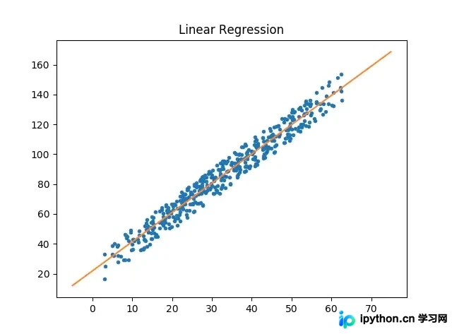
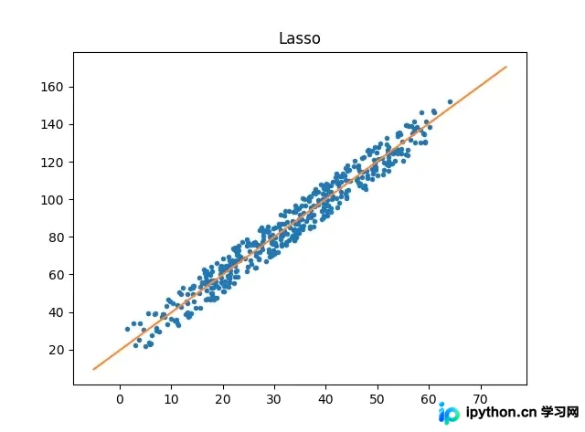
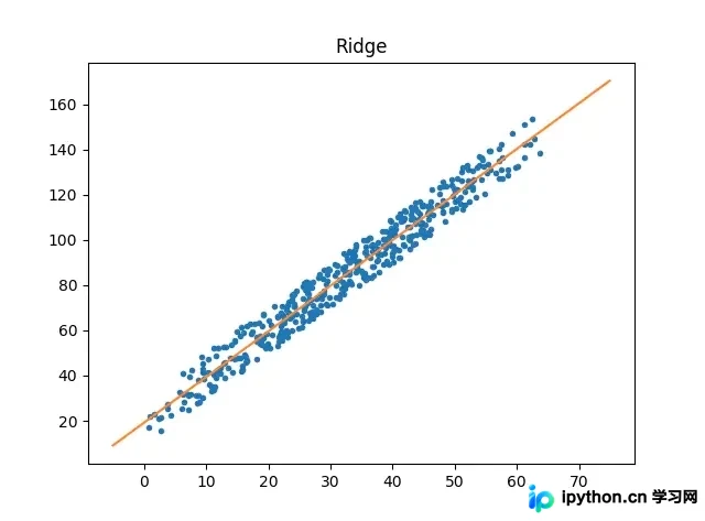
测试代码部分包含数据生成函数 gen_reg_data 及三个测试函数。gen_reg_data 生成 0 到 45 范围内的特征 X，并添加随机噪声，目标变量 y 由 2*X 加上噪声和常数 10 构成。test_linear_regression、test_lasso 和 test_ridge 分别实例化对应模型，拟合数据后使用 matplotlib 绘制散点图及预测直线，并显示图表标题。


import matplotlib.pyplot as plt
import numpy as np

def gen_reg_data():
 X = np.arange(0, 45, 0.1)
 X = X + np.random.random(size=X.shape[0]) * 20
 y = 2 * X + np.random.random(size=X.shape[0]) * 20 + 10
 return X, y

def test_linear_regression():
 clf = LinearRegression()
 X, y = gen_reg_data()
 clf.fit(X, y)
 plt.plot(X, y, '.')
 X_axis = np.arange(-5, 75, 0.1)
 plt.plot(X_axis, clf.predict(X_axis))
 plt.title("Linear Regression")
 plt.show()

def test_lasso():
 clf = Lasso()
 X, y = gen_reg_data()
 clf.fit(X, y)
 plt.plot(X, y, '.')
 X_axis = np.arange(-5, 75, 0.1)
 plt.plot(X_axis, clf.predict(X_axis))
 plt.title("Lasso")
 plt.show()

def test_ridge():
 clf = Ridge()
 X, y = gen_reg_data()
 clf.fit(X, y)
 plt.plot(X, y, '.')
 X_axis = np.arange(-5, 75, 0.1)
 plt.plot(X_axis, clf.predict(X_axis))
 plt.title("Ridge")
 plt.show()